
Passive cavity aerosol spectrometer probe (PCASP) Calibrations and Performance Checks
UND Performance Check Documentation:
Concentration Calibrate (Aerosol Flow Rate)
1) Turn on the PCASP pump by connecting the black control box to the instrument and flip the switch to the On position. Use a flow standard, such as the Gilibrator. Use the smallest Gilian container and connect tube to the bottom hole (see picture below).

2) Measure the concentration at the exit of the flow system (see picture below)

3) Use the black button by the tube to take 6 samples with the Gilibrator and the average flow rate should be around 60 ccm.
Sizing Calibration
Note that the calibration is for one refractive index and size. Typically, there will be particles from other sizes due to not having pure (ultra clean works best) water or reusing the nebulizers. The best method to clean the nebulizers is to rise them with pure (distilled) water many, many times. Helps to store the nebulizers in distilled water and seal the nebulizers.
- Make sure all equipment in the system (pump, laser, m300 computer, etc.) is turned on (see picture below)
- Note the size of the beads used for the calibration
- Clean solution container with distilled water to avoid contamination
- Record data using the M300 or M200 Data Acquisiion System
- Check that the counts are zero when beginning (performance check)
- This ensures the filter is working properly with no major leaks in the system
- Upload the data and process using the ADPAA software.
- Analyze the result using the ADPAA software.
 Image showing size performance check.
ADPAA Processing of PCASP Performance Checks

- Open the document that contains the table with calibration information and enter the date for a given PCASP calibration into the table. I will be referring to the Saudi Arabia 222 nm calibration from 3/10/08 in the steps to follow. See the table and graphs below.
- In a terminal find the “date”.counts.pcasp.raw for the PCASP calibration data. The path for the Saudi Arabia 3/10/08 calibration is /nas/2008/08_03_10.
- Open the “date”.readme file.
- Scroll to find the PCASP information. For this case, Saudi 3/10/08, you will find a TEST 1 and TEST 2 (two calibrations were done on the PCASP that particular day.)
- Note that TEST 1 is .222 um. Enter this into the calibration table under the Size column. Be sure to pay attention to the units (um or nm). For the .222 um calibration, the “date”.readme file states that it began at approximately 12:18 and stopped at 12:37. Also, it says there was a peak in Channel 5. (You may want to keep this .readme file open or make note of the start time, end time, and peak channel.) Keep in mind that the times in this readme file are approximate; we will use cplot to find the specific time interval of the calibration.
- In a terminal, run
$ time_convert.tcl
A small window will open allowing you to convert seconds from midnight (sfm) to hour:min:sec or back to sfm. Convert the approximate start and end times to sfm.
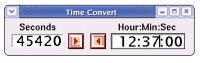
Make note of them because they will help us in cplot. For this example, the approximate start time is 44280 and end time, 45420.
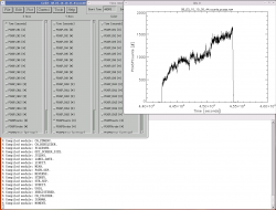
- Back in the terminal with the raw data ( /nas/2008/08_03_10/ ), open the “date”.counts.pcasp.raw file with cplot,
$ cplot 08_03_10_10_35_44.counts.pcasp.raw
- Plot Time vs. PCASPCounts.
- X-axis → Time
- Y-axis → PCASPCounts
- Click Plot → XY Graph.
- For this particular day, two PCASP calibrations were performed. To ensure we isolate TEST 1, the .222 um case, we will use the approximate start and end times we found in the “date”.readme file.
- The object is to narrow down the graph to find a specific start time and end time which will isolate only the peak due to the beads during calibration. In this example, with 44280 and 45420 being our approximate start and end times, I started by cutting the time interval down from 44200 to 45600.
- To change the Time Interval of the graph, click Control → Time Interval. Enter a Start and End Time and press ENTER (or cplot will not recognize the interval change.)
- Re-plot the graph by clicking Plot → XY Graph. You should see a zoomed in graph that should be isolated around the peak (due to the beads going through the PCASP during calibration.)
- Using Time Interval feature, find a specific start and end time.
- TIP: Try isolating just the beginning of the peak. In this 3/10/08 case, I first narrowed my graph from 44100 to 44300, then narrowed a bit further until finding a start time of 44240. Do the same for the end of the peak.
- Once you are satisfied with a start time and an end time, enter these times into the calibration table. See table below.
- Still in cplot, be sure your Time Interval is set to the start and end time you chose. Click Plot → Spectrum. This plots the number of counts in each channel. With this example, we confirm that the peak is in Channel 5. Enter this peak channel into the table. Shown below is the Spectrum and the XY Graph.
- The table asks for Pre-Peak, Peak, and Post-Peak Counts. To find these using cplot, keep the Time Interval the same. Click Edit → Options → Display Text. Plot the Spectrum again. This time a text window will open with the spectrum graph, giving the counts in each channel. Record the Pre-Peak, Peak, and Post-Peak Counts into the table as shown below. For example, the peak was in Channel 5, we we want the counts in Channels 4, 5, and 6.
- The last step is finding the average channel in which the beads were sized. In a terminal, run
$ avg_channel
It will prompt you for the Peak Channel as well as the Pre-Peak, Peak, and Post-Peak Counts, which you found using cplot. It will give you the average channel, which you can enter into the table.


3/10/08 PCASP Calibration Checks - Saudi Arabia
| Date | Size (nm) | Start Time (sfm) | End Time (sfm) | Peak Channel | Average Channel |
|---|---|---|---|---|---|
| 3/10/08 | 222 | 44246 | 45450 | 5 | 5.059135 |
| 3/10/08 | 532 | 45992 | 46273 | 8 | 7.889956 |
222 nm 3/10/08 Calibration - Spectrum (left) and XY Graph (right)


Click on an image to enlarge.
532 nm 3/10/08 Calibration - Spectrum (left) and XY Graph (right)


Click on the image to enlarge.
Processing Calibration Data:
- In a terminal, use the ADPAA script process_raw to process and convert the *.sea file recorded with the data system.
- Use the ADPAA cplot to determine the time period of the bead test.
- Use the cplot <Edit><Options> window and turn on 'Display Text'. Plot a spectrum and note the calculated 'Chn Avg' value in the Text Window.
- Use the ADPAA program setprobes_pcasp to calculate the channel boundaries using the average channel value determine for the Cplot analysis.